Neural Networking using Python

A neural network is a method in artificial intelligence that teaches computers to process data in a way that is inspired by the human brain. It is a type of machine learning process, called deep learning, that uses interconnected nodes or neurons in a layered structure that resembles the human brain.
What are neural networks used for?
Neural networks have several use cases across many industries, such as the following:
Medical diagnosis by medical image classification
Targeted marketing by social network filtering and behavioral data analysis
Financial predictions by processing historical data of financial instruments
Electrical load and energy demand forecasting
Process and quality control
Chemical compound identification
How to train neural networks?
Neural network training is the process of teaching a neural network to perform a task. Neural networks learn by initially processing several large sets of labeled or unlabeled data. By using these examples, they can then process unknown inputs more accurately.
Supervised learning
In supervised learning, data scientists give artificial neural networks labeled datasets that provide the right answer in advance. For example, a deep learning network training in facial recognition initially processes hundreds of thousands of images of human faces, with various terms related to ethnic origin, country, or emotion describing each image.
The neural network slowly builds knowledge from these datasets, which provide the right answer in advance. After the network has been trained, it starts making guesses about the ethnic origin or emotion of a new image of a human face that it has never processed before.
Building a Neural Network
We will be focusing on building a neural network using Python Programming.
The first step in building a neural network is generating an output from input data. We’ll do that by creating a weighted sum of the variables. The first thing you’ll need to do is represent the inputs with Python and NumPy.
We can use an IPython console or a Jupiter Notebook to follow along. It’s a good practice to create a new virtual environment every time we start a new Python project, so you should do that first.
We will first have to activate the virtual environment.
$ python -m venv ~/.my-env
$ source ~/.my-env/bin/activate
Using the above commands, we first create the virtual environment, then we activate it. Now it’s time to install the IPython console using pip. Since we’ll also need NumPy and Matplotlib, it’s a good idea install them too:
(my-env) $ python -m pip install ipython numpy matplotlib
(my-env) $ ipython
Now you’re ready to start coding.
Now, we will train a model to make predictions that have only two possible outcomes. The output result can be either 0 or 1. This is a classification problem, a subset of supervised learning problems in which we have a dataset with the inputs and the known targets. These are the inputs and the outputs of the dataset:
| Input Vector | Target |
| [1.66, 1.56] | 1 |
| [2, 1.5] | 0 |
The target is the variable you want to predict. In this example, we’re dealing with a dataset that consists of numbers. This isn’t common in a real production scenario. Usually, when there’s a need for a deep learning model, the data is presented in files, such as images or text.
Making Your Prediction
Let us keep things straightforward and build a network with only two layers. For a network with multiple layers, there would always be a network with fewer layers that predicts the same results.
What we want is to find an operation that makes the middle layers sometimes correlate with an input and sometimes not correlate.
We can achieve this behavior by using nonlinear functions. These nonlinear functions are called activation functions. There are many types of activation functions. The ReLU(rectified linear unit), for example, is a function that converts all negative numbers to zero. This means that the network can “turn off” a weight if it’s negative, adding nonlinearity.
The network you’re building will use the sigmoid activation function. You’ll use it in the last layer, layer_2. The only two possible outputs in the dataset are 0 and 1, and the sigmoid function limits the output to a range between 0 and 1. This is the formula to express the sigmoid function:

The e is a mathematical constant called Euler’s number, and we can use np.exp(x) to calculate eˣ.
Probability functions give you the probability of occurrence for possible outcomes of an event. The only two possible outputs of the dataset are 0 and 1, and the Bernoulli distribution is a distribution that has two possible outcomes as well. The sigmoid function is a good choice if your problem follows the Bernoulli distribution, so that’s why you’re using it in the last layer of your neural network.
Since the function limits the output to a range of 0 to 1, we’ll use it to predict probabilities. If the output is greater than 0.5, then you’ll say the prediction is 1. If it’s below 0.5, then you’ll say the prediction is 0. This is the flow of the computations inside the network you’re building:
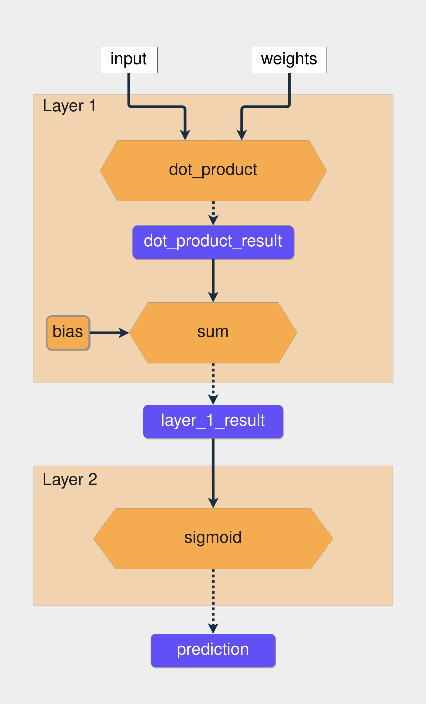
The yellow hexagons represent the functions, and the blue rectangles represent the intermediate results. Now it’s time to turn all this knowledge into code. We’ll also need to wrap the vectors with NumPy arrays. This is the code that applies the functions presented in the image above:
 # Wrapping the vectors in NumPy arrays
 input_vector = np.array([1.66, 1.56])
 weights_1 = np.array([1.45, -0.66])
 bias = np.array([0.0])

 def sigmoid(x):
       return 1 / (1 + np.exp(-x))

 def make_prediction(input_vector, weights, bias):
        layer_1 = np.dot(input_vector, weights) + bias
        layer_2 = sigmoid(layer_1)
        return layer_2

 prediction = make_prediction(input_vector, weights_1, bias)

 print(f"The prediction result is: {prediction}")

#OUTPUT
 The prediction result is: [0.7985731]
The raw prediction result is 0.79, which is higher than 0.5, so the output is 1. The network made a correct prediction. Now try it with another input vector, np.array([2, 1.5]). The correct result for this input is 0. We’ll only need to change the input_vector variable since all the other parameters remain the same:
 # Changing the value of input_vector
 input_vector = np.array([2, 1.5])

 prediction = make_prediction(input_vector, weights_1, bias)

 print(f"The prediction result is: {prediction}")

#OUTPUT
 The prediction result is: [0.87101915]
This time, the network made a wrong prediction. The result should be less than 0.5 since the target for this input is 0, but the raw result was 0.87.
Conclusion
We built a neural network from scratch using NumPy. With this knowledge, you’re ready to dive deeper into the world of artificial intelligence in Python.
The process of training a neural network mainly consists of applying operations to vectors. Today, you did it from scratch using only NumPy as a dependency. This isn’t recommended in a production setting because the whole process can be unproductive and error-prone. That’s one of the reasons why deep learning frameworks like Keras, PyTorch, and TensorFlow are so popular.